
A scanning laser vibrometer can map ultrasonic vibration across a small specimen without attaching a sensor to each measurement point. In this case, a fixed laser vibrometer provided a vibration-response reference while a gimbal scanning head measured nine positions on an approximately 20 × 10 mm specimen. Analysis in the 20–50 kHz band produced two EFDD modal candidates and a separate operating deflection shape (ODS). Their different quality indicators show why a spectral peak and a clear deformation image require different engineering interpretations.
This technical case explains the acquisition arrangement, the reported results and the checks needed before using those results for a design decision. Customer identity is omitted. The figures reproduce the original test photograph and software outputs.
Why use a scanning laser vibrometer for ultrasonic vibration?
For a small component, an attached accelerometer and its mounting can change the dynamics being measured. Optical measurement avoids sensor mass loading at the specimen’s scan points and leaves the measurement surface accessible. Scanning adds spatial information: instead of observing one response trace, the engineer can compare motion at different positions and visualize a sampled deformation pattern.
The benefit depends on the test conditions. Optical return, spot placement, measurement direction, fixture behavior and reference stability remain important. The scan grid describes positions on a surface; it does not turn a single line-of-sight laser measurement into a three-component displacement vector. For background, see the laser Doppler vibrometer measurement principle.
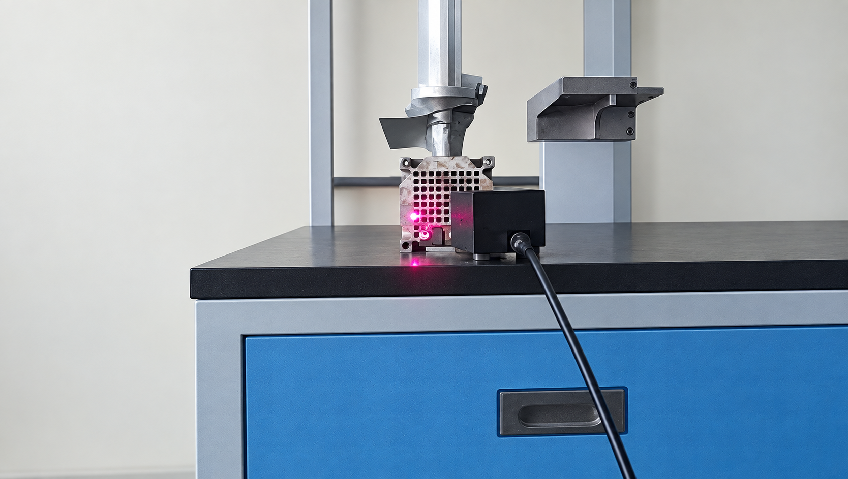
Test setup: a fixed response reference and nine scan points
The experiment used two acquisition channels. AIN3 recorded the fixed vibration-stage response, while AIN2 recorded the specimen response sequentially at nine positions. Both channels were acquired together at each scan position. The fixed reference provides a common basis for comparing scans, provided the operating condition remains sufficiently stable throughout the sequence.
| Item | Recorded setting |
|---|---|
| Specimen dimensions | Approximately 20 × 10 mm |
| Spatial measurement | Nine sequential scan points, represented on a two-dimensional surface topology |
| Fixed reference | AIN3, vibration-stage response |
| Scanning response | AIN2, specimen response |
| Sampling rate | 256 kHz |
| OMA analysis band | 20–50 kHz |
| Identification method | Enhanced Frequency Domain Decomposition (EFDD) |
The reference is a measured response, not an excitation-force input. This distinction matters when interpreting the H1 estimate used for the ODS comparison. It is a response-to-response relationship in this experiment, rather than a force-normalized mechanical frequency response function.
The 256 kHz sampling rate is a recorded test setting, not a statement of the instrument’s usable measurement bandwidth. The acquisition chain also needs suitable analog bandwidth and anti-alias filtering. Record length and spectral processing determine frequency resolution, which is particularly important for narrow peaks and low damping estimates.
EFDD results in the 20–50 kHz analysis band
Operational modal analysis (OMA) estimates modal properties from measured responses without requiring a measured force input. Frequency Domain Decomposition uses the response spectral density matrix and its singular values to help separate modal contributions. EFDD extends this approach with a selected modal spectral region to estimate frequency and damping. The result still depends on excitation, data quality and the validity of the identification assumptions.
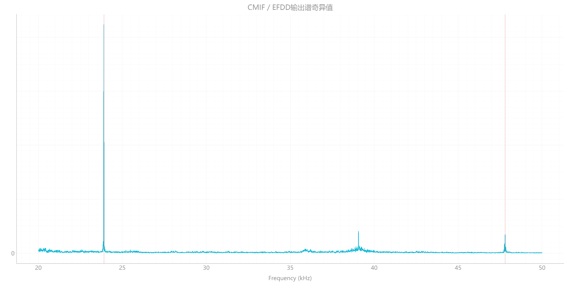
| Result | Frequency (Hz) | MPC | Reported damping (%) | Interpretation |
|---|---|---|---|---|
| EFDD candidate 1 | 23,902.415 | 0.871 | 0.012 | High-confidence candidate in the source report; engineering verification remains necessary. |
| EFDD candidate 2 | 47,803.030 | 0.471 | 0.010 | Candidate requiring manual review and repeat measurement. |
| Frequency-slice ODS | 24,078.125 | 0.984 | Not reported | Operating response shape at the selected frequency, not an independently confirmed mode. |
Modal Phase Collinearity (MPC) describes phase collinearity of a complex shape vector. It provides useful quality evidence, but it is not a probability that a mode is correct. The source also reports Mean Phase Deviation (MPD) values of 7.214° and 19.530° for the first and second candidates, respectively. The second candidate has lower phase consistency and deserves closer inspection.
The damping percentages above are the algorithm’s reported estimates. They should not be treated as validated material constants or guaranteed structural damping values without reviewing the record length, leakage, frequency resolution and excitation conditions.
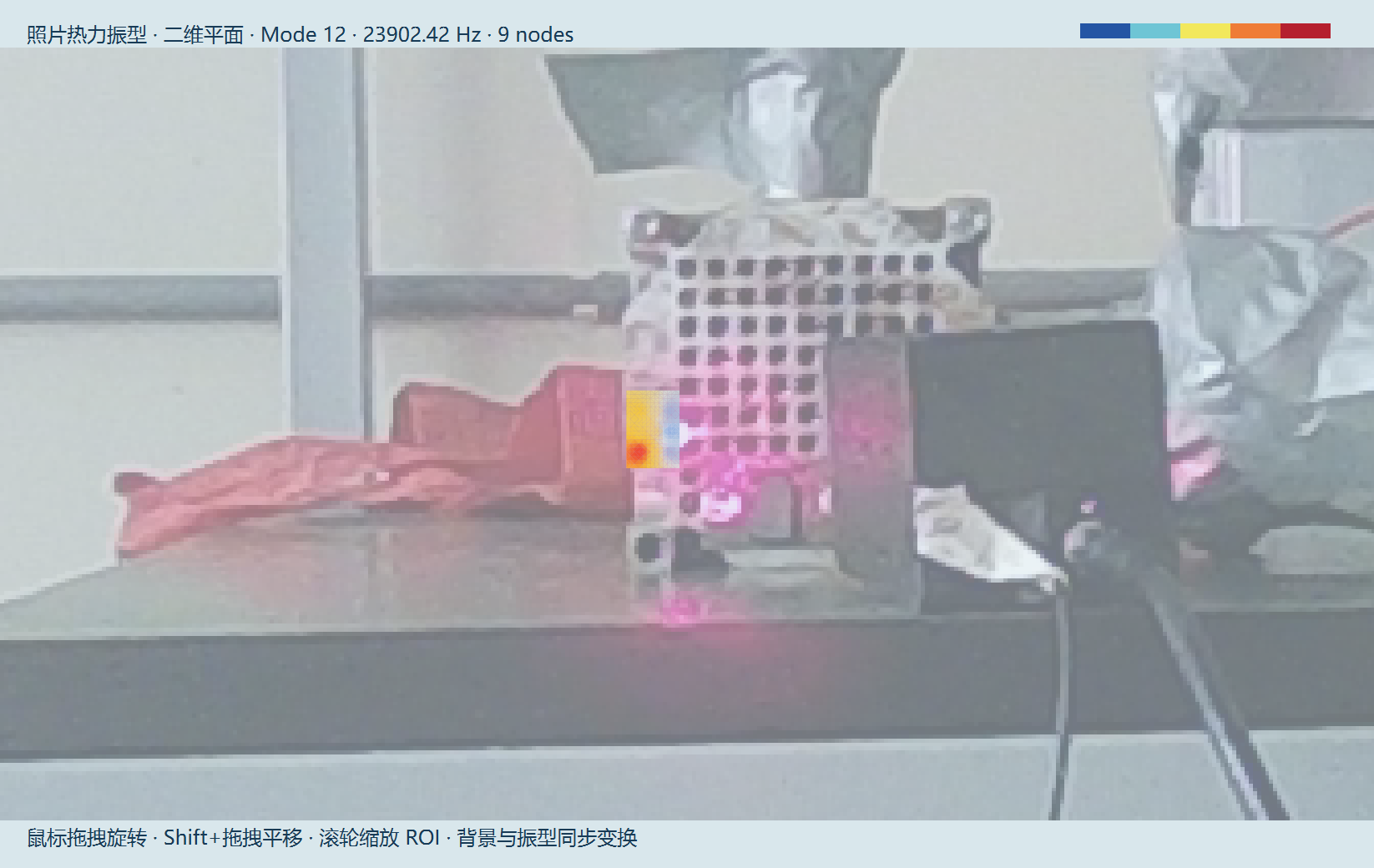
Candidate shape at 23,902.415 Hz
Candidate shape at 47,803.030 Hz
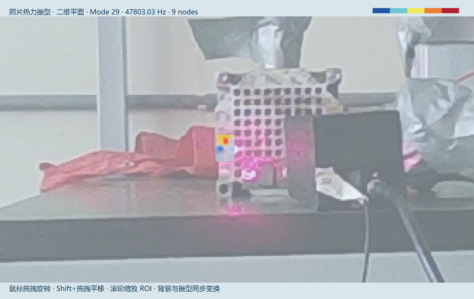
The report gives a cross-correlation value of 0.017 between these candidate vectors in its Auto-MAC matrix. This indicates low correlation for those sampled vectors. It does not independently prove that both candidates are genuine structural modes, particularly with only nine spatial samples.
An additional check follows directly from the reported frequencies: 47,803.030 Hz is very close to twice 23,902.415 Hz. This near 2:1 relationship warrants a harmonic-content check; it does not by itself identify the second feature as either a harmonic or a structural mode. Literature on EFDD under deterministic excitation explains why harmonic components can interfere with modal extraction [1]. The available case results do not establish that such interference has been removed.
ODS at 24,078.125 Hz: the operating response shape
The ODS calculation combines the fixed response reference and the scanning response using an H1 estimate. It shows the relative spatial response at 24,078.125 Hz under the recorded operating condition. Its MPC value of 0.984 indicates strong phase collinearity for that shape, but does not convert an operating response into a confirmed natural mode.
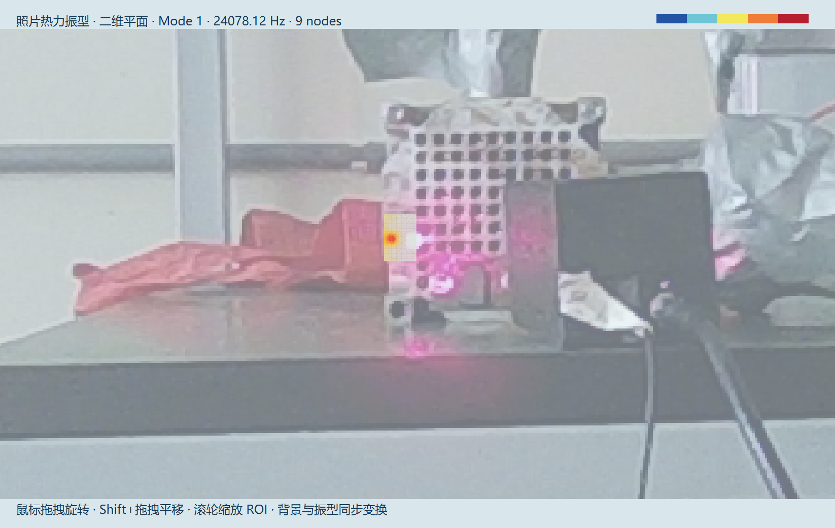
The ODS frequency is close to the first EFDD candidate, but frequency proximity alone cannot establish modal equivalence. A comparison needs compatible measurement coordinates and directions, consistent normalization, and matching operating conditions. The distinction is explained further in ODS, OMA and EMA method selection.
What the case supports and how to verify the candidates
The case demonstrates a non-contact measurement route for spatial ultrasonic response visualization and candidate-mode identification on a small specimen. The fixed-reference arrangement connects the sequential scans to a common response baseline. The nine-point grid makes the results interpretable spatially, while the quality indicators keep uncertain candidates visible rather than silently treating every peak as a confirmed mode.
Nine points remain a sparse sample. Interpolation between them does not add measured spatial detail, and finer localized patterns may require a denser grid. Gimbal positioning therefore needs to be checked against the specimen dimensions, spot size and expected shape complexity. It is the laser acquisition bandwidth, not the mechanical scan speed, that must capture the ultrasonic response at each stationary measurement point.
- Repeat the acquisition. Compare both candidate frequencies and shapes across repeat runs, prioritizing the 47.803 kHz region.
- Check reference and optical quality. Confirm reference stability, spot placement, surface return and absence of clipping or signal dropout.
- Review excitation content. Inspect possible harmonics, including the near 2:1 frequency relationship, before assigning modal significance.
- Review processing and spatial coverage. Record acquisition duration, spectral resolution and processing settings. Increase point density where the sampled shape needs more detail.
- Corroborate the interpretation. Where feasible, use independent excitation or a measured-force modal test, and compare with an appropriate model. Keep ODS displays separate from validated modal parameters.
The current results do not establish a fault type, fatigue life, stress field or pass/fail quality threshold. Those decisions require additional measurement and validation.
Frequently asked questions
Can a scanning laser vibrometer measure ultrasonic vibration?
Yes, when the optical sensor, acquisition chain and analysis settings support the required frequency range and signal level. This case reports a 256 kHz sampling rate and analysis from 20 to 50 kHz. Those settings do not guarantee equivalent results on a different specimen or instrument configuration.
Why use a fixed laser vibrometer alongside a scanning head?
The fixed response channel provides a common reference for sequential scan measurements. Stable operating conditions and sufficient reference signal are necessary for meaningful amplitude and phase comparison. It does not replace a measured force input when a force-normalized FRF is required.
Does high MPC prove that an ultrasonic peak is a natural mode?
No. MPC describes phase collinearity, not a calibrated confidence probability. Repeatability, excitation content, spatial coverage and independent verification also matter. Even the high-confidence candidate in this report remains a candidate until engineering validation.
Can the 24.078 kHz ODS be used as the first modal shape?
It should be reported as the operating deflection shape at 24,078.125 Hz. Its relationship to the 23,902.415 Hz EFDD candidate requires further comparison. The software’s Mode 1 display label does not establish a first natural mode.
Are nine scan points sufficient for every small ultrasonic specimen?
No. Point density should follow the geometry and the spatial variation of interest. Nine points supported the sampled displays in this case, but cannot resolve every local deformation feature or establish a strain field on their own.
Sources and related measurement resources
Case evidence: the September 2026 ultrasonic vibration-stage OMA/ODS technical presentation and its accompanying technical article. Numerical values in this page reproduce the reported results. The setup photograph, EFDD spectrum and shape screenshots come from the presentation; no curves or quality states have been redrawn. Customer identity is omitted.
[1] Jacobsen, N.-J., Andersen, P. and Brincker, R. (2007). Using EFDD as a Robust Technique for Deterministic Excitation in Operational Modal Analysis. Proceedings of the 2nd International Operational Modal Analysis Conference, pp. 193–200. This source supports the harmonic-interference discussion, not the case’s numerical results.
For system planning, review the VP-PVM-100 gimbal scanning laser vibrometer and the non-contact modal testing workflow. Optical access, spot placement and bandwidth should be assessed for the actual specimen before selecting a measurement configuration.