
Technical review: Mr. Sun, Technical Manager
Summary: A scanning laser vibrometer supports blade fault detection by combining non-contact multi-point response measurements with modal frequency, damping, mode-shape and MAC comparisons. The method can reveal repeatable structural differences, but it does not identify a crack or fault type without repeat testing and physical inspection.
How scanning measurement supports blade fault detection
A scanning laser vibrometer supports blade fault detection by measuring vibration response at multiple points without adding sensor mass. The resulting frequency response functions provide natural frequencies and damping estimates, while the spatial response grid reconstructs mode shapes. Engineers can then compare matched modes with the Modal Assurance Criterion, or MAC, instead of relying on frequency shifts alone.
This distinction matters because a changed resonance does not identify a fault by itself. Fixture stiffness, preload, excitation position, optical return and analysis settings can also move a peak or alter damping. A defensible diagnosis first confirms that two results represent the same mode, then checks whether the difference repeats under controlled conditions.
Why blade measurements need spatial information
Blades are light, thin and often curved. Their higher-order bending and torsional modes can be closely spaced, and an accelerometer may influence a local response through its mass, cable force or adhesive layer. A laser Doppler vibrometer avoids this mechanical loading by measuring surface motion along the optical line of sight.
A single-point laser vibrometer remains useful for screening. It can locate resonant peaks and estimate natural frequency and damping from a local frequency response function. Its limitation appears when two peaks overlap, a response point lies near a modal node, or modal order changes between tests. In those cases, the frequency sequence does not prove mode identity.
A scanning laser vibrometer adds the missing spatial evidence. The scanner moves the measurement beam across a defined grid and records amplitude and phase at each point. Modal analysis software uses these responses to reconstruct operating deflection shapes or mode shapes. Engineers can compare how the structure deforms, not only where a spectral peak appears.
Single-point screening and multi-point confirmation
| Method | Primary output | Best use | Important limit |
|---|---|---|---|
| Single-point identification | Local frequency and damping | Fast screening and threshold monitoring | No mode-shape evidence; nearby peaks can be mismatched |
| Multi-point identification | Frequency, damping and mode shape | Confirming mode identity and spatial changes | Grid, direction, boundary and reference must be consistent |
| MAC | Mode-shape correlation from 0 to 1 | Comparing matched spatial patterns | Not a health score or damage probability |
| Subspace correlation | Correlation with a candidate modal space | Checking mixed modes or competing matches | A larger subspace naturally raises correlation |
Measurement workflow for blade comparison
The test begins with equivalent boundary conditions. Both blades should use the same fixture, installation datum, preload and excitation position. Root constraints have a strong effect on blade dynamics, and damping is especially sensitive to friction at the interface.
The scan grid should cover the root, airfoil body and tip. Points across the chord help resolve torsional motion, while points along the span describe bending. Corresponding point numbers, locations and measurement directions must remain consistent between samples. For curved blades, the optical line-of-sight direction should also be recorded so that any geometric compensation can be reviewed.
Experimental modal analysis normally uses an impact hammer or shaker as the force reference. Because a gimbal scanning laser vibrometer acquires response points sequentially, a stable force or response reference preserves phase relationships across the grid. Without a reliable reference, amplitude trends may still be useful, but a complex mode shape cannot be reconstructed with confidence.
Data quality review comes before curve fitting. The operator should examine optical return, overloads, double hits, coherence, force-spectrum coverage and repeatability. A common reference cannot correct a test in which the structure, excitation or optical condition changes substantially during the scan.
A and B blade comparison
The supplied comparison contains nine corresponding measurement points on Blade A and Blade B. Both datasets were evaluated with H1 frequency response functions over 70 to 3000 Hz using the same modal-identification settings. The values below come from the raw-data re-identification and therefore may differ slightly from historical screenshots produced with earlier fitting settings.
| Candidate match | Blade A | Blade B | Frequency change | Complex MAC | Interpretation |
|---|---|---|---|---|---|
| Low-order group | 496.63 Hz / 1.652% | 499.42 Hz / 0.765% | +0.56% | 0.993 | Clear spatial match |
| High-frequency candidate 1 | 2345.51 Hz / 0.479% | 2476.38 Hz / 0.141% | +5.58% | 0.833 | Related; pairing not final |
| High-frequency group | 2623.91 Hz / 0.202% | 2747.32 Hz / 0.337% | +4.70% | 0.983 | Clear spatial match |
| High-frequency candidate 2 | 2345.51 Hz / 0.479% | 1954.87 Hz / 0.401% | -16.65% | 0.716 | Partial shared shape |
Interpretation note: MAC values compare spatial mode-shape similarity. They are not health scores or probabilities of damage.
What the modal correlation means
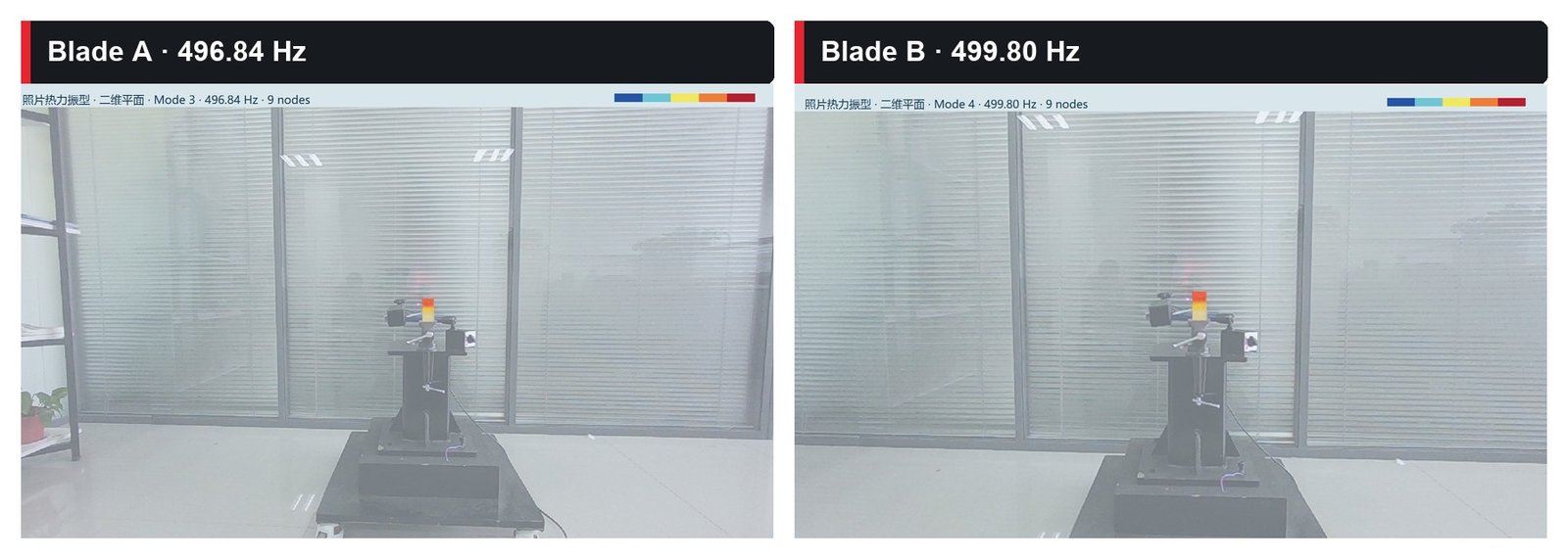
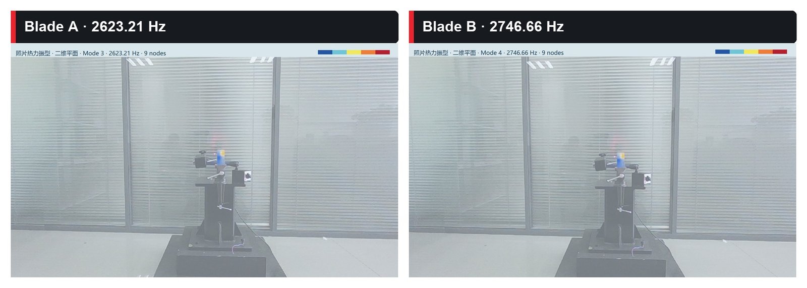
The low-order modes show a clear match. Their complex MAC is 0.993 and the frequency shift is 0.56%. The modes near 2624 Hz and 2747 Hz also correlate strongly, with a MAC of 0.983, although their frequency difference is larger.
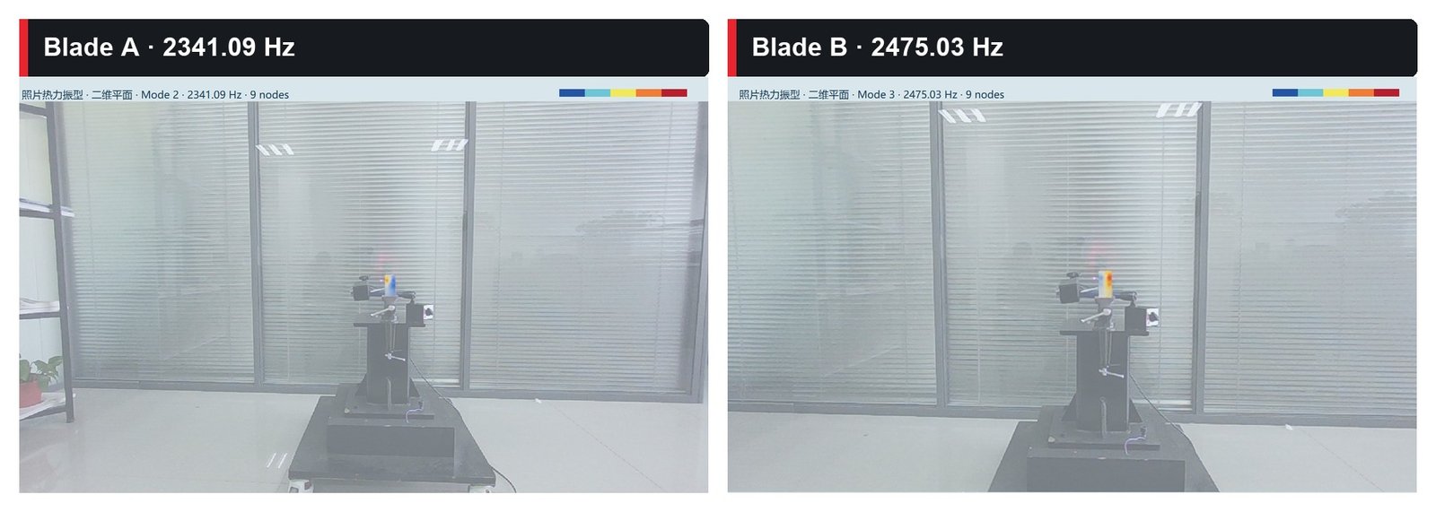
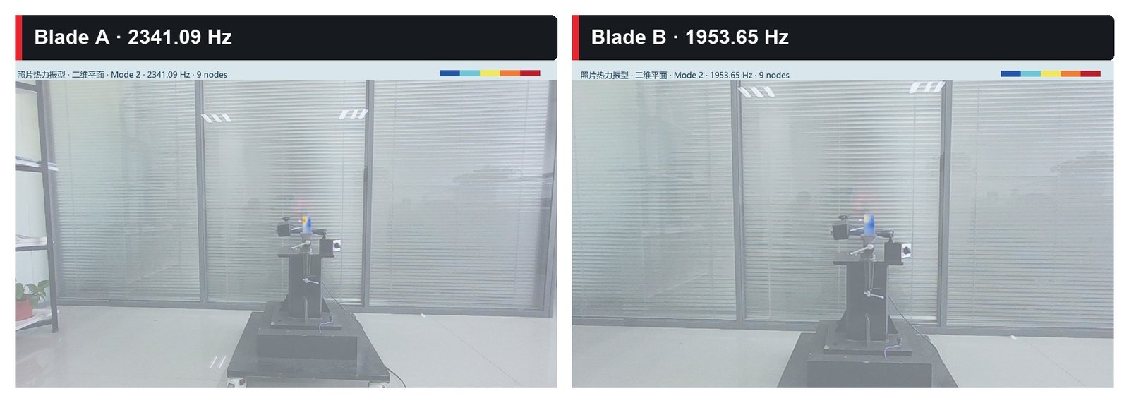
The mode near 2345.51 Hz on Blade A produces a less certain result. It correlates with a 2476.38 Hz mode on Blade B at 0.833 and retains some similarity with a 1954.87 Hz candidate at 0.716. Changing the maximum fitting order can reverse the ranking of these two candidates. A frequency-only comparison could therefore assign the wrong counterpart.
A subspace comparison provides additional context. When the 1955 Hz and 2476 Hz candidates on Blade B are treated as a two-dimensional modal subspace, the Blade A mode correlates with that subspace at 0.916. The result stays between 0.916 and 0.920 across the tested fitting orders. This supports the interpretation that the original spatial pattern may be distributed across two candidates. It does not mean that there is a 91.6% probability of damage.
Mode-shape images make the correspondence visible
The following images come from the supplied Blade A and Blade B comparison document. Each view displays the spatial vibration pattern reconstructed from nine measurement points. Color and deformation indicate the relative response pattern used for modal comparison; they are not stress maps, crack maps or direct images of damage.
The frequencies printed in these visualization results differ slightly from the raw-data re-identification values in the table above because the images were generated in a separate fitting run with different analysis settings. The engineering interpretation therefore uses the raw-data table for numerical comparison and the images for spatial evidence.
Can the result prove modal splitting or blade damage
The data justify further investigation, but they do not identify a specific defect. Several mechanisms can produce the observed competition. Blade A may contain a weak neighboring mode that the original excitation did not reveal. Structural differences may change modal coupling. Fixture stiffness, preload, impact position, optical return or model order may change observability. Local stiffness loss, looseness, geometric variation or mass redistribution may also mix or separate modes.
The two Blade B candidates are about 522 Hz apart, so they do not form a typical pair of narrowly separated peaks. Before calling the result damage-induced modal splitting, the test team should search the same band on Blade A for a weaker second mode and confirm that both Blade B candidates remain stable after re-clamping, changing the excitation position and varying the reasonable fitting order.
From anomaly detection to fault attribution
A practical blade fault detection program uses modal parameters as evidence, not as a stand-alone diagnosis. The first stage monitors stable peaks at fixed points. The second stage scans the blade when a frequency, damping or response change exceeds the established repeatability band. Mode shapes, MAC, Auto-MAC and stabilization diagrams then determine whether the same physical mode has changed.
Repeated tests complete the statistical check. If the modal difference persists, engineering inspection can focus on the affected region and use dimensional measurement, material records, visual inspection, ultrasonic testing or computed tomography to identify the cause. This sequence separates a repeatable dynamic signature from fixture variation and links the vibration result to physical evidence.
Where a gimbal scanning laser vibrometer fits
A gimbal scanning laser vibrometer is well suited to stationary blade tests that require a broad measurement field, longer stand-off distance or a scan surface that cannot carry many sensors. It supports development modal validation, sample-to-sample comparison, repair verification, finite-element model correlation and detailed review of an abnormal blade.
The method is less efficient when the only objective is an online limit check at one stable point. A fixed single-point laser vibrometer can perform that task faster. Sequential scanning also assumes that the structure and excitation remain stationary during acquisition. Transient or rapidly changing operating conditions require synchronized multi-point measurements or another validated reference strategy.
VIPICO’s PVM-100 scanning laser vibrometer combines gimbal point positioning with non-contact response acquisition and modal-analysis workflows. The selection of grid density, frequency range, excitation and reference channels should follow the blade geometry, expected modes, working distance and test duration.
Frequently Asked Questions
Can a scanning laser vibrometer locate a blade crack directly?
A single modal test cannot identify an exact crack location with certainty. Frequency, damping and mode-shape changes can identify a structural difference and guide denser scanning or nondestructive inspection.
Does a higher MAC mean the blade is healthier?
No. MAC measures spatial similarity between two mode shapes. A high value means the shapes are similar. A low value may indicate a structural change, a mismatched mode or poor data quality.
Why can frequency-only blade fault detection fail?
Modal order can change, neighboring modes can overlap and one test may excite a mode more strongly than another. Mode-shape matching should establish the physical correspondence before frequency and damping are compared.
Can damping alone diagnose blade damage?
Damping is sensitive to fixture friction, preload, temperature, excitation amplitude, windows and fitting range. It works best as a supporting feature whose repeatability has been measured.
Are more scan points always better?
The grid should resolve the highest mode of interest. Too few points miss local behavior. Excessive density increases scan time and exposure to drift or changing optical return.